语义分割代码阅读

2024-06-04 14:04| 来源: 网络整理| 查看: 265

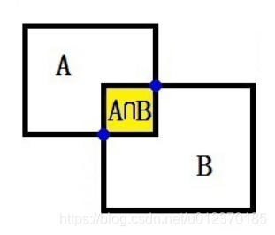
1. 语义分割IoU的定义传统意义上的IoU(Intersection over Union，交并比)

直观表示:

公式: $S_{A\bigcup B}=S_A+S_B-S_{A\bigcap B}$

语义分割中的IoU

在语义分割的问题中，这两个集合为真实值（ground truth）和预测值（predicted segmentation）。这个比例可以变形为正真数（intersection）比上真正、假负、假正（并集）之和。在每个类上计算IoU，之后平均。

å¨è¿éæå¥å¾çæè¿°

语义分割中的MIoU

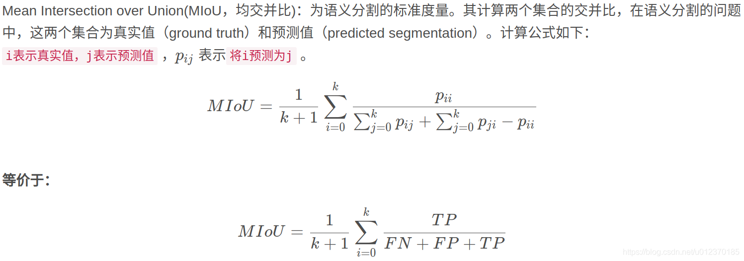
Mean Intersection over Union(MIoU，均交并比)：为语义分割的标准度量。其计算所有类别交集和并集之比的平均值.

2. 某个类别的IoU的计算

对于pascal数据集来说, 对于21个类别, 分别求IOU: 对于某一个类别的IOU计算公式如下:

直观理解:

å¨è¿éæå¥å¾çæè¿°

MIoU：计算两圆交集（橙色部分）与两圆并集（红色+橙色+黄色）之间的比例，理想情况下两圆重合，比例为1。

扩展提示: TP(真正): 预测正确, 预测结果是正类, 真实是正类 FP(假正): 预测错误, 预测结果是正类, 真实是负类 FN(假负): 预测错误, 预测结果是负类, 真实是正类

TN(真负): 预测正确, 预测结果是负类, 真实是负类 #跟类别1无关,所以不包含在并集中 (本例中, 正类:是类别1, 负类:不是类别1)

扩展阅读:

准确率和召回率

3. mIoU的计算

对于每个类别计算出的IoU求和取平均

步骤一先求出混淆矩阵

步骤二再求MIoU

混淆矩阵的每一行再加上每一列，最后减去对角线上的值

import numpy as np class IOUMetric: """ Class to calculate mean-iou using fast_hist method """ def __init__(self, num_classes): self.num_classes = num_classes self.hist = np.zeros((num_classes, num_classes)) def _fast_hist(self, label_pred, label_true): # 找出标签中需要计算的类别,去掉了背景 mask = (label_true >= 0) & (label_true < self.num_classes) # # np.bincount计算了从0到n**2-1这n**2个数中每个数出现的次数，返回值形状(n, n) hist = np.bincount( self.num_classes * label_true[mask].astype(int) + label_pred[mask], minlength=self.num_classes ** 2).reshape(self.num_classes, self.num_classes) return hist # 输入：预测值和真实值 # 语义分割的任务是为每个像素点分配一个label def ev aluate(self, predictions, gts): for lp, lt in zip(predictions, gts): assert len(lp.flatten()) == len(lt.flatten()) self.hist += self._fast_hist(lp.flatten(), lt.flatten()) # miou iou = np.diag(self.hist) / (self.hist.sum(axis=1) + self.hist.sum(axis=0) - np.diag(self.hist)) miou = np.nanmean(iou) # -----------------其他指标------------------------------ # mean acc acc = np.diag(self.hist).sum() / self.hist.sum() acc_cls = np.nanmean(np.diag(self.hist) / self.hist.sum(axis=1)) freq = self.hist.sum(axis=1) / self.hist.sum() fwavacc = (freq[freq > 0] * iou[freq > 0]).sum() return acc, acc_cls, iou, miou, fwavacc 项目中的代码: class Evaluator(object): def __init__(self, num_class): self.num_class = num_class self.confusion_matrix = np.zeros((self.num_class,)*2)#21*21的矩阵,行代表ground truth类别,列代表preds的类别,值代表 ''' 正确的像素占总像素的比例 ''' def Pixel_Accuracy(self): Acc = np.diag(self.confusion_matrix).sum() / self.confusion_matrix.sum() return Acc ''' 分别计算每个类分类正确的概率 ''' def Pixel_Accuracy_Class(self): Acc = np.diag(self.confusion_matrix) / self.confusion_matrix.sum(axis=1) Acc = np.nanmean(Acc) return Acc ''' Mean Intersection over Union(MIoU，均交并比)：为语义分割的标准度量。其计算两个集合的交集和并集之比. 在语义分割的问题中，这两个集合为真实值（ground truth）和预测值（predicted segmentation）。这个比例可以变形为正真数（intersection）比上真正、假负、假正（并集）之和。在每个类上计算IoU，之后平均。对于21个类别,分别求IOU: 例如,对于类别1的IOU定义如下: (1)统计在ground truth中属于类别1的像素数 (2)统计在预测结果中每个类别1的像素数 (1) + (2)就是二者的并集像素数(类比于两块区域的面积加和, 注:二者交集部分的面积加重复了) 再减去二者的交集(既在ground truth集合中又在预测结果集合中的像素),得到的就是二者的并集(所有跟类别1有关系的像素:包括TP,FP,FN) 扩展提示: TP(真正): 预测正确, 预测结果是正类, 真实是正类 FP(假正): 预测错误, 预测结果是正类, 真实是负类 FN(假负): 预测错误, 预测结果是负类, 真实是正类 TN(真负): 预测正确, 预测结果是负类, 真实是负类 #跟类别1无关,所以不包含在并集中 (本例中, 正类:是类别1, 负类:不是类别1) mIoU: 对于每个类别计算出的IoU求和取平均 ''' def Mean_Intersection_over_Union(self): MIoU = np.diag(self.confusion_matrix) / ( np.sum(self.confusion_matrix, axis=1) + np.sum(self.confusion_matrix, axis=0) - np.diag(self.confusion_matrix)) MIoU = np.nanmean(MIoU) #跳过0值求mean,shape:[21] return MIoU def Class_IOU(self): MIoU = np.diag(self.confusion_matrix) / ( np.sum(self.confusion_matrix, axis=1) + np.sum(self.confusion_matrix, axis=0) - np.diag(self.confusion_matrix)) return MIoU def Frequency_Weighted_Intersection_over_Union(self): freq = np.sum(self.confusion_matrix, axis=1) / np.sum(self.confusion_matrix) iu = np.diag(self.confusion_matrix) / ( np.sum(self.confusion_matrix, axis=1) + np.sum(self.confusion_matrix, axis=0) - np.diag(self.confusion_matrix)) FWIoU = (freq[freq > 0] * iu[freq > 0]).sum() return FWIoU ''' 参数的传入: evaluator = Evaluate(4) #只需传入类别数4 evaluator.add_batch(target, preb) #target:[batch_size, 512, 512] , preb:[batch_size, 512, 512] 在add_batch中统计这个epoch中所有图片的预测结果和ground truth的对应情况, 累计成confusion矩阵(便于之后求mean) 参数列表对应: gt_image: target 图片的真实标签 [batch_size, 512, 512] per_image: preb 网络生成的图片的预测标签 [batch_size, 512, 512] parameters: mask: ground truth中所有正确(值在[0, classe_num])的像素label的mask---为了保证ground truth中的标签值都在合理的范围[0, 20] label: 为了计算混淆矩阵, 混淆矩阵中一共有num_class*num_class个数, 所以label中的数值也是在0与num_class**2之间. [batch_size, 512, 512] cout(reshape): 记录了每个类别对应的像素个数,行代表真实类别,列代表预测的类别,count矩阵中(x, y)位置的元素代表该张图片中真实类别为x,被预测为y的像素个数 np.bincount: https://blog.csdn.net/xlinsist/article/details/51346523 confusion_matrix: 对角线上的值的和代表分类正确的像素点个数(preb与target一致),对角线之外的其他值的和代表所有分类错误的像素的个数 ''' # 计算混淆矩阵 def _generate_matrix(self, gt_image, pre_image): mask = (gt_image >= 0) & (gt_image < self.num_class)#ground truth中所有正确(值在[0, classe_num])的像素label的mask label = self.num_class * gt_image[mask].astype('int') + pre_image[mask] # np.bincount计算了从0到n**2-1这n**2个数中每个数出现的次数，返回值形状(n, n) count = np.bincount(label, minlength=self.num_class**2) confusion_matrix = count.reshape(self.num_class, self.num_class)#21 * 21(for pascal) return confusion_matrix # -------------------------------------------------------------------------------- def add_batch(self, gt_image, pre_image): assert gt_image.shape == pre_image.shape tmp = self._generate_matrix(gt_image, pre_image) #矩阵相加是各个元素对应相加,即21*21的矩阵进行pixel-wise加和 self.confusion_matrix += self._generate_matrix(gt_image, pre_image) def reset(self): self.confusion_matrix = np.zeros((self.num_class,) * 2)

其中, 利用计算出来的混淆矩阵计算MIoU的方法如下:

''' confusion_matrix是一个[num_classes,num_classes]的矩阵, confusion_matrix矩阵中(x, y)位置的元素代表该张图片中真实类别为x,被预测为y的像素个数第一个MIoU: [bach_size, 类别数]:对角线/(混淆矩阵各行加和+各列加和-对角线) 第二个MIoU: [1, 类别数] ''' def Mean_Intersection_over_Union(self): MIoU = np.diag(self.confusion_matrix) / ( np.sum(self.confusion_matrix, axis=1) + np.sum(self.confusion_matrix, axis=0) - np.diag(self.confusion_matrix)) MIoU = np.nanmean(MIoU) #跳过0值求mean,shape:[1, 21] return MIoU

后面是用fake数据帮助理解,可忽略:

其中a:预测值, b: ground truth

>>> b array([[0, 0, 0, 2], [0, 0, 2, 1], [1, 1, 1, 0], [1, 0, 1, 2]]) >>> a array([[0, 0, 0, 2], [0, 0, 2, 1], [1, 1, 1, 2], [1, 0, 1, 2]]) >>> label = 3 * b[mask] + a[mask] >>> count = numpy.bincount(label) >>> count array([6, 0, 1, 0, 6, 0, 0, 0, 3]) >>> count = count.reshape(3, 3) >>> numpy.sum(count, axis=1) array([7, 6, 3]) >>> numpy.sum(count, axis=0) array([6, 6, 4]) >>> numpy.sum(count, axis=1) + numpy.sum(count, axis=0) array([13, 12, 7]) >>> numpy.sum(count, axis=1) + numpy.sum(count, axis=0) - numpy.diag(count) array([7, 6, 4])

参考链接: https://blog.csdn.net/baidu_27643275/article/details/90445422

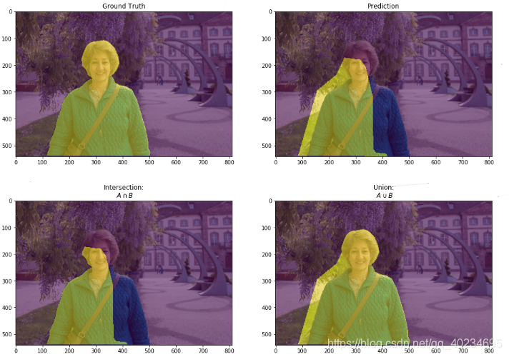
【本文地址】

公司简介

联系我们